A single value to measure equity market correlation

There exists a vast amount of studies that show an increase in correlation between global equity indices during bear markets and propose ways to measure/forecast this correlation (see for example Campbell, Koedjik and Kofman or Capiello, Engle and Sheppard, and many, many more). These studies differ greatly in their methodologies and complexities but they more or less all show the same significant increase in correlation during downturns in the equity market.

In this post we will take a look at a very simple method of measuring this correlation and using it to produce a market strength signal.

As a single-value metric to measure the general correlation inbetween different equity markets we will use the so-called “Standardized Generalized Variance”, or SGV for short. Generalized Variance was introduced by Wilks in Contributions to Probability and Statistics and adapted to SGV by Gupta.

What makes SGV so appealing is that it conveniently summarizes the information contained in the variance-covariance matrix for a given set of returns in one single number that can also be compared between different return matrices. For example, it would be possible to compare SGV values of equity and bond markets, or compare correlations inbetween different regions.

For a given m * n dimensional matrix of log returns, SGV is defined as taking the n-th root of the determinant of the variance-covariance matrix of log returns, or  where  is the covariance matrix of log returns.

For the return data we will be using a set of ETFs covering the major global equity markets (this is a simplifying assumption but using ETFs traded at the same exchange allows circumventing the time asynchronicity between indices; a way for accounting for this asynchronicity would for example be using the Hayashi-Yoshida correlation estimator and constructing based on that).

The chosen ETFs are VTI (US Total Stock Market), EZU (iShares MSCI Eurozone), EWJ (iShares MSCI Japan) and EEM (iShares MSCI Emerging Markets).

Let’s take a look at the 1 year rolling SGV.

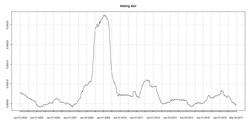
A few interesting features are immediately visible from this chart. First, the run up in the SGV prior to the Financial Crisis and the extreme spike caused by it. Second, also a run up (although less pronounced) can be observed before the Euro Debt Crisis in 2011.

Now overlay the mean returns of the chosen ETFs with the SGV to take a closer look.

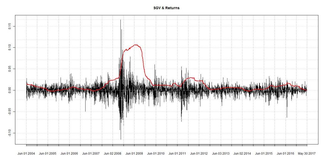
This emphasizes the observations from before. SGV seems to do a reasonable job of identifying big run ups in correlation and therefore downturns in the equity market.

So how is this usable or in any way helpful? In it’s raw form SGV can extend the range of market strength indicators as well as risk measures. It can be part of a system identifying regime changes in the market as well as a signal for the need of downside protection. It could also build the basis of a trading strategy.

As a very simplified example, let’s have a look at the performance of a trading strategy that goes long VTI whenever the current SGV is below its 6 month high and switches to bonds (TLT) when it reaches a new high.

This is by no means a properly thought out and well constructed trading strategy, it just serves the purpose of demonstrating the fact that it definitely has merit spending some time on investigating the properties and possibilities of SGV further. This, however, will be the topic of a future post.

Until then,

QUANTBEAR

APPENDIX:

For running this code I used timeseries collected in my personal database. As the current Yahoo Finance data situation is not very good (understatement), I will only present the implementation of the SGV calculation (which is really straightforward anyway and can easily be translated to other programming languages). Once I find a suitable replacement for free EOD data, I will upload the full code to my github.

#obtain your matrix of log returns
cov_mat <- cov(logRet)

getSGV <- function(covv){
    det(covv)^(1/ncol(covv))
}

SGV <- getSGV(cov_mat)