Food for thought: Risk Backtesting?

As you are reading this blog you are definitely familiar with the concept of backtesting trading strategies, and probably have done so a significant amount of times. But do you also backtest your risk metrics? They are as important of a building block of your portfolios overall performance as the trading strategies themselves. So if you are not backtesting your VaRs and Expected Shortfalls (not a comprehensive list), I hope that this post will show you that it is quite necessary. In case you are a risk metric backtesting guru already, maybe you can still find some things useful (or point out flaws and make me learn something new!).

*Disclaimer: The following concepts and techniques will be explained using VaR. I am well aware that it is not the only risk measure (but it still is the most common one) and also that it has severe limitations and drawbacks (it is not even a coherent risk measure). However, since this post is supposed to provide you with food for thought instead of a ready-to-use implementation, I think it is sufficient. Future posts will be concerned with building upon what is presented here (and hopefully what will be added through a discussion in the comments) and moving towards a sophisticated, professional risk management system for our portfolio.

All that being said, let’s get started. Our asset of choice for this exercise will be a classic, the S&P500 ETF or SPY. We will look at different implementations to obtain the 1-day 95% VaR. But before we get into that, lets define the criteria for our VaR backtest. What we want to obtain is a risk measure that contains next day’s return in 95% of the cases. In the other 5%, where return is lower than our VaR, we get an exception.

In the case that our model is perfect, the number of exceptions follows a binomial distribution with a mean of n*p and a standard deviation of . Given our confidence level of 95% (p = 5%) and 250 trading days a year, this would result in an expected number of exceptions of 12.5 ± 3.44. So our exceptions on a rolling 250-day basis should lie between 9 and 16.

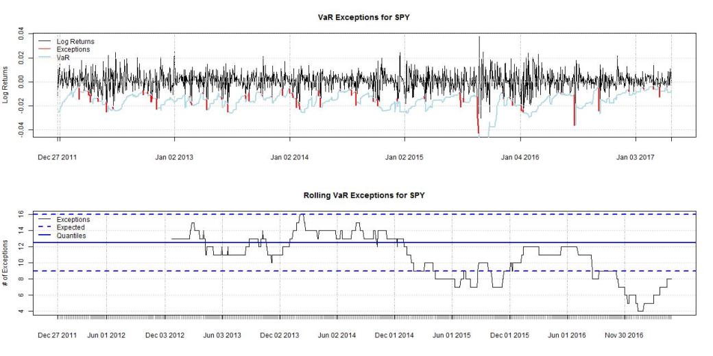
First, let’s have a look at a parametric VaR. We use a 2-year lookback window to estimate the mean and standard deviation and obtain the VaR over the sample period (the always excellent QuantStart has an article about VaR in general and specially this approach).

The results are not very satisfying to say the least. We have long periods of no exceptions at all followed by very poor performance during the financial crisis. So it seems we need to try a different approach. Let’s see how historical simulation would have performed, again using the returns over the last 2 years. In this method, a set of past returns is used to obtain an approximation to the theoretical distribution, and the quantile value is taken to obtain the VaR.

Looks quite similar to before, again a very poor performance. It is apparent that our implementations are not adapting fast enough (or not at all) to changes in the market environment. As the next step, we try to weight the returns used in historical simulation by their age, weighing more recent returns higher than older ones. For this we use the following exponential weighting function:

with . After obtaining the new distribution of returns, we take the quantile again to obtain the VaR. With this approach, we try to make our risk metric more adaptable to changing market conditions. The results are more promising:

We can see that the VaR is adjusting better to changes and also during the crisis we don’t have such a high number of exceptions anymore. But can we still improve this? Instead of weighting the returns by their age, we try weighing them by the volatility in the market. We use the 20day standard deviation to normalize each return and multiply each return in the lookback period by the corresponding volatility to obtain the new distribution.

This method seems to be sometimes better, sometimes worse than age weighting. So a logical idea would be to combine those methods! We firstly normalize all returns again by dividing through the volatility, weighting them by their age and lastly multiplying them by the current volatility measure (as an extra layer of protection instead of taking the last value we take the max over the last 20days) to obtain our return distribution.

Now this looks much better! Our returns are below the upper quantile during the whole backtesting horizon. It is a very conservative approach, but better safe than sorry.

As a final step, let’s check how our VaR metric would have performed out of sample.

Also in the out-of-sample horizon this implementation would have performed very well.

So what was the point of all this? First and foremost, it is well worth it to spend some effort on backtesting your risk metrics. It is also important to keep an open mind and critically think about how and why you move to different implementations.

Again, let me emphasize that this whole exercise is to get the general idea across. Neither VaR itself, nor any of these implementations and parameters used are “the best solution”, they merely serve as a starting point for thinking about backtesting risk metrics. In upcoming posts I will be discussing specific risk metrics (and their implementations) in much more detail. As always I am interested in hearing your thoughts about this topic in general.

Until next time,

QUANTBEAR

PS: The implementations of the methods used are fairly straightforward, I will not post them here since the code is not the main point of the post. It is however available on request in either R or Python.