Risk Premia Market Timing?

Here it goes, finally a strategy backtest (sort of) on this blog (what an intro).

In their 1973 paper “Risk, Return and Equilibrium: Empirical Tests”, Fama and MacBeth introduce a method for estimating betas and risk premia for any risk factors that determine asset prices. Under the assumption that the only common risk factor that drives asset prices is the market itself, we will use their method, the Fama-MacBeth regression, to obtain an estimate of the current overall risk premium and use it for market timing (again, sort of).

In this regression method there are essentially two steps that need to be performed:

1. regress each asset against the risk factor to obtain each asset’s beta
2. regress all asset returns in a given time period against the betas to obtain the risk premium for that factor

The main hypothesis that we will use is that when we obtain a positive risk premium it is a good indicator to be long the market as we get compensated for taking risk (we will not care about the size of premium) and when premium is negative, we move to cash (in our case the SHY ETF).

As the code used for this strategy will be focused on immediate reproducability, some simplifying assumptions have to be made:

• as the market risk factor we will use the S&P500 returns
• the assets used are 250 stocks that were part of the S&P at the beginning and end of the backtest (using only these stocks we introduce a somewhat significant survivorship bias, however in my opinion this can be neglected as this serves only as a demonstration; I am also aware that not everyone has a survivorship-bias free database of stock prices and historical compositions which would make it hard to reproduce the results presented here)
• the backtest will start from 2002 onwards (decimalisation for US stocks was introduced in April 2001, electronic trading also really took off with the start of the new millenium and I am somewhat reluctant to run these super-long backtests for times when basically everything was different [funny thing to say when using a paper from 1973 though]), and again, reproducability

The first thing that we will take a look at is using the assumption of the betas being fixed. So we only perform step 1 of the regression method onceand use the resulting betas over the whole insample backtest window. We will use 3 years of daily return data to estimate the betas (Fama and MacBeth use 4 – 5 years of monthly return data) and then use the resulting values to estimate the daily risk premia. Averaging those over a rolling 1-year time window we obtain the current expected risk premia in the market. The resulting equity curve is as follows:

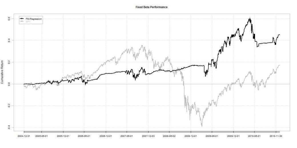
Over the tested period this produces the following metrics:

• Annualized Return            6.4 %
• Annualized Std               10.95 %
• Max Drawdown:            16.61 %
• Annualized Sharpe              0.58

The two things that are immediately visible from the comparison to the SPY etf are that the strategy produces a higher terminal value than the SPY and that all of that outperformance is achieved during the financial crisis. So far the use as a standalone strategy seems rather limited, at best it might be used as some sort of risk gauge.

But what happens if we choose a different calibration window for the betas? We will still use the assumption that the betas stay fixed but now we will use a 1-year window.

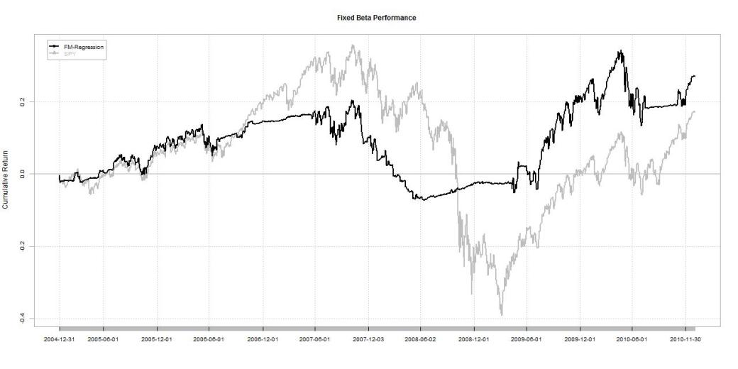
• Annualized Return           4.05 %
• Annualized Std               11.55 %
• Max Drawdown:            23.03 %
• Annualized Sharpe              0.35

Ok this is clearly worse. And many of you will immediately say: “are you just trying random parameters and now and see what works?” No, I am trying to emphasize a striking difference between the two strategy returns. For the first 15months, the second implementation outperforms the first and is on par with the market. The difference here is that the betas were estimated “closer” to that period. So the logical jump that we will make here is: rolling beta estimation!

We will estimate betas now on a rolling 1 year basis for every day and obtain the risk premia in the same way as before.

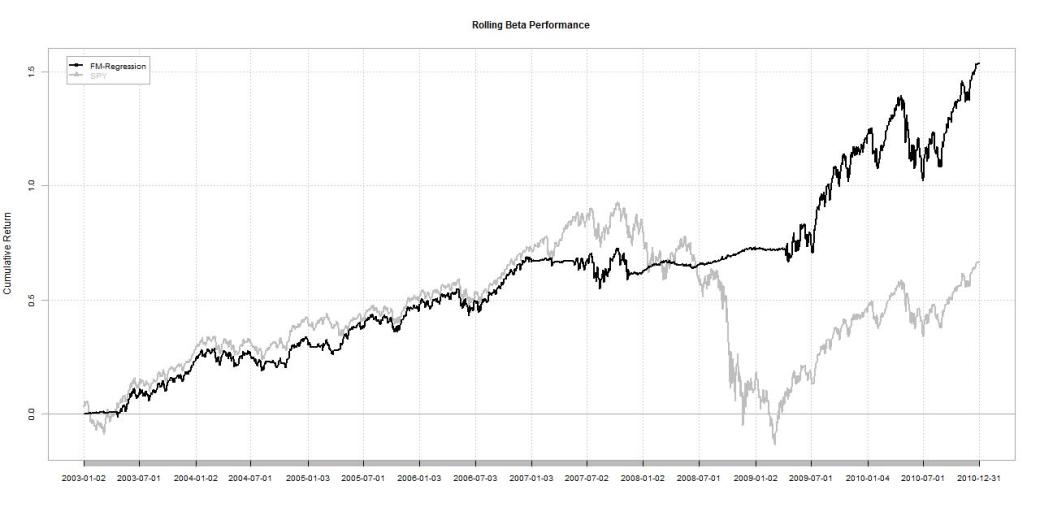
• Annualized Return         12.33 %
• Annualized Std                12.12 %
• Max Drawdown:              15.69 %
• Annualized Sharpe             1.02

Ok, now we’re talking. That looks like something that can be of use. We slightly lag the market but make up for it through an early switch to cash before the financial crisis. Not too bad for timing the market!

Let’s see if the results also hold up out of sample:

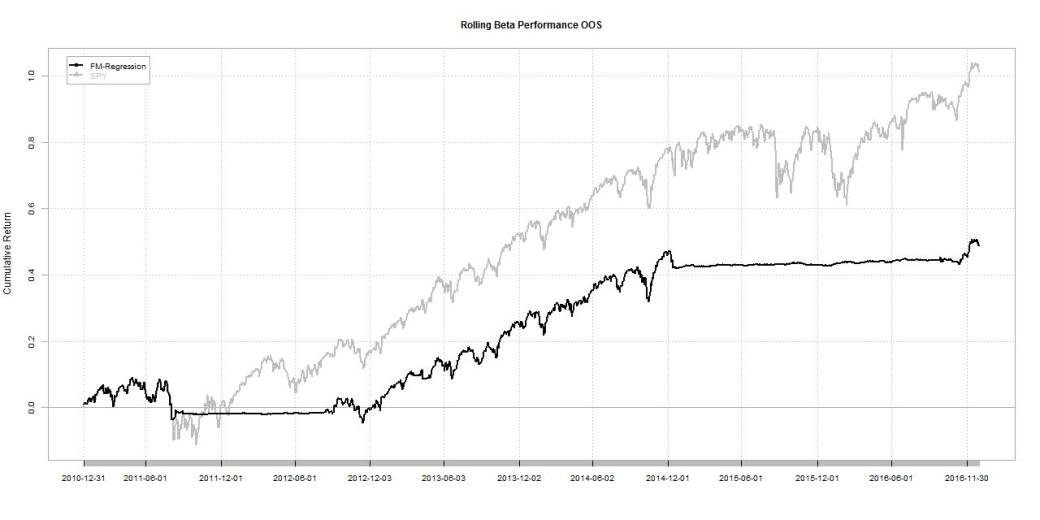
Not that impressive. We manage to evade the zig-zagging of 2015 and early 2016 but apart from that we lag behind the market return significantly.

So what’s the takeaway? It seems that using this method to estimate risk premia can serve as some sort of a market timing strategy. I would not recommend this as a standalone strategy (see out of sample results), however using it to complement your existing portfolio and/or using it as a risk gauge definitely has some merit. Also moving into some other asset than cash when the premium is negative (bonds come to mind) can be effective.

I’ll end this post with the following disclaimer:

• Don’t trade this (at least not in this form)!
• Be aware of the assumptions I made when running this test (see above). I know that using only a subset of stocks introduces a bias but again, reproducability.
• Don’t trade this (at least not in this form)!

I would definitely be happy to discuss this method in more detail as I have only recently began toying around with it. So please drop your thoughts in the comments.

Until next time,

QUANTBEAR

PS: You can find the R implementation here